Games Of Chance

In this post we’ll discuss games with elements of uncertainty.

Games of chance have a distinctive place in the theory of probability because of its close ties with gambling.
There is however an important distinction to be made.
Games such as Roulette, Craps or ‘Snakes and Ladders’ can be deemed “boring” because they are memoryless i.e your future success has no dependence on how the game was played in the past, only on where you are currently (so they resemble Markov Chains).
In addition these games have no intermediate decision making so in summary we may safely claim there is no skill involved.

Other games such as Poker and Bridge involve uncertainty and imperfect information but are generally considered games of skill partly because it is possible to distinguish between good and bad decisions and choosing between them requires skill.

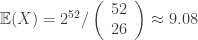
Of course games like poker depend on so much more than just probabilistic decision making. It also involves things like psychology, emotional control and exploitation of your opponents tendencies. In recent time there has been great dispute in many courts as to whether poker is a game of inherent skill or a game of pure luck. The distinction has great legal (and reputational) implications, since games that are considered gambling are usually only allowed in casinos. For example the federal judge in New York last year ruled that poker is indeed a game of skill, partly because the opposition failed to convincingly explain why so many players who had been identified as winners/losers after a certain number of hands, kept on consistently winning/losing over time. The moral being you would not be able to make such two-sided predictions from a random walk. One of the charts shown to the judge may be viewed in this article.

Below you can see a simple Excel simulation of how the casino edge plays out in a game of Red/Black Roulette-betting over 10,000 spins. The chart shows the 5 best and the 5 worst paths out of an initial population of 100. Each bet is 1$.

Here of course everyone will lose money eventually because the game is not fair (expected value is -0.027$/spin with a 1$ bet).
The point is that you cannot predict future success for say the purple player after observing 1,000 spins, despite the player seemingly beating the game at that point (not knowing the rest of the story).

It is not always obvious determining whether a game requires skill, and if so, what strategies are most favourable.
Here are a few interesting made-up games that illustrate this.

Problem 1 (Game Show):

Suppose you are part of a game show and have just received the chance to win a car.

There are three doors.
Behind two of them is a goat, and behind the remaining door you will find the car.
The host lets you choose one door after which he proceeds to open a different door.
It turns out that the door opened by the host had a goat behind it.
The host now offers you to keep the door you have or switch.

What should you do?

Solution:

This is a bit of a trick question if you have the relevant background on this game.

The game is actually not in your favour and requires no skill in the sense that all strategies have equal probability of winning the car.

Did you think this was the classic Monty Hall problem?
Actually it isn’t because you were never told what the show host was going to do and hence there is no conditional probability involved. The door that was opened turned out to have a goat behind it.
In general you need to know the protocol of the host to derive probabilistic information. If you don’t know then the chances are plain and simple.

For those of you who were not caught by this and have not heard of Monty Hall before I recommend you read the wikipedia article in the link above.
If you know that the host is going to show you a goat after choosing your door then things change.
Your chances of winning by switching will then have increased to .
This version of the game appeared on an actual TV show called Let’s Make a Deal which mainly aired on NBC for many years.

 

I once heard a story (though sounding more like an urban legend) regarding a candidate interviewing for a role at a wall street investment bank, offered to play the same game as above except the prize was different (and no, the interviewer did not use goats).
If the candidate won he would immediately advance to the final round for this highly competitive job, otherwise he would have to go home.
The candidate having heard about the Monty Hall problem confidently accepted because he did not estimate his chances of advancing to exceed .
According to the story the interviewer told the candidate to step outside the room while he put a coin under one of three paper cups. When the candidate was called back he chose the wrong cup. The interviewer then revealed the coin under a different cup and told the candidate to go home. The candidate was confused and started arguing that an empty cup was supposed to be revealed. The interviewer merely stated that they were looking for candidates who could pay attention to details while under high pressure…

The next two games are related to guessing the colour of the next card in a deck.
Let’s investigate if the games are “boring” or whether there exist any good strategies.

Problem 2 (Red Or Black? – Version 1):

Given is a perfectly shuffled deck of playing cards (26 Black, 26 Red).

Each card is revealed to you one by one, and at any point in time you can stop the dealer and bet 1$ on the next card being Red.

You are allowed to bet only once throughout the game and if you don’t bet you are automatically betting 1$ on the last card (so you are effectively paying 1$ to play the game).

If you win you get back 2$.

What would be your best strategy?

Solution:

It sounds like you should be able to gain an advantage by waiting for the number of Red cards in the deck to exceed the number of Black cards and then bet, but of course that may never happen and then you will lose in the end.

It turns out this game is fair and no matter what strategy you chose you can never gain an advantage but also never lose any advantage.

This is actually an immediate consequence of the Martingale Stopping Theorem which (in this context) says that the chance of winning by betting at the very beginning is the same as the chance of winning by betting at any other time (in expectation). In probability theory Martingales are essentially models of fair games. Your winning probability in this game is a discrete-time martingale.

There is however a much nicer argument.
Suppose you have some arbitrary strategy.
Instead of betting on the next card being Red you bet on the last card being Red.
At any point during the game the probability of the next card being Red is of course the same as the probability of the last card being Red, so the two versions of the game are equivalent. But this new version is completely uninteresting because you win anyway if the last card is Red regardless of the strategy you chose i.e the last card doesn’t change just because you choose a different strategy.

 
 

The next game is much more interesting and now the question is instead how much money you can make.

Problem 3 (Red Or Black? – Version 2):

Again a dealer perfectly shuffles a standard deck of 52 cards with equally many Red and Black cards.

You start with 1$.

The dealer turns over one card at a time and gives you the opportunity to bet any fraction of your current worth on the colour of the next card.

The dealer gives you even odds on every bet, meaning he will return you double the bet if you win regardless of the composition of the deck.

Clearly you can wait and bet nothing until the last card when you are guaranteed to win
and go home with 2$.

The question is if you can do any better, and if so, what is the maximum guaranteed amount you can leave with?

Solution:

Consider the following “suicide” strategy:
Suppose you take for granted that the colours in the deck are distributed in some specific way and bet everything you have that the cards will follow that fixed distribution on every turn.

In the unlikely event that you don’t go broke your fortune will be massive, namely dollars.

Despite this, the expected return of the strategy (mathematically speaking) is
dollars since any of the other remaining distributions will leave you with dollars.

Suppose you clone yourself into mini-me’s that each play this game following the same strategy using a different fixed distribution out of the possible.

Any strategy must amount to splitting up your initial worth between the clones in some way.
To see this suppose your strategy entails betting dollars on Red on the first turn.
Then you split dollars equally between the clones that bet on Red and split dollars equally among the clones betting on Black on the first turn. You then continue distributing the remaining part of your dollar in the same way by adding funding to the surviving clones according to your strategys decision tree.
In the end every clone has it’s own stake of the initial dollar.

Thus any strategy is composed of some funding allocation of dollars to each clone where .

The expected return of the strategy is therefore given by where is the random variable for the return of clone starting with dollar.
Each of the clones have the same expected return so .
We therefore get .

Hence remarkably it does not matter how the money is initially split between the clones as every such strategy have the same expected value. In particular every such strategy is optimal in expectation.

We can now guarantee ourselves of receiving the expected return by dividing the initial dollar equally among all clones. This way we know that one of them will get the distribution right and hence survive all the way through with total expected return of .

Since we can never guarantee anything better than the expected return this is the best possible guaranteed return.

 

The above argument shows that exactly one of the clone players will have assumed the correct deck colour distribution starting with dollars.
That players wealth will therefore grow like .

In practise you can only make one bet per card so you would then simply look at the net bet made by all clones and adopt that bet for yourself. That means an aggregated bet of dollars on Red and dollars on Black among the clones, amounts for you to a bet of dollars on Red if and dollars on Black if .

 
The last game I wanted to discuss may also seem intuitively surprising.

You may have seen the classic cult movie Highlander from 1986. If you haven’t it’s not that important, it’s mainly about violent Scottish swordsmen who are hunting each other down to gain each others powers.

Problem 4 (There Can Be Only One):

The Macleods and the Frasers are two Highlander clans (and sworn enemies).

They have currently spotted each other somewhere in Glenfinnan on the shores of Loch Shiel in the Highlands of Scottland.

The members of the Macleod clan have strengths and the Frasers have strength .

The Highlanders fight one-on-one until death, two people at a time.

If two Highlanders, one with strength battles a Highlander with strength then the former wins with probability and the latter with probability .

Once a Highlander cuts off the head of another Highlander the winner must yell “There can be only one!!!” and will then gain the strength of the killed Highlander.

After each match, the Frasers put forward a combatant of their choosing among those still alive in the clan, and the Macleods do the same right behind.

The winning clan is the clan that remains alive with at least one person.

Do the Macleods have a favourable strategy, getting to put forward their candidate last?

Solution:

Interestingly the game is actually fair.

To see this note that each individual combat is fair in the sense that the expected gain or loss of strength in each combat is zero for both clans:
.

Let be the probability that Macleods win the battle.
If they win they would of course have accumulated all Frasers strength into their clan and if they lose they will have given away their total accumulated strength, leaving them with no strength.
Therefore since Macleods are not expected to gain any strength over the course of the battle we get:

Hence the probability of winning is for Macleods regardless of lineup.

 
 

Why not you try below problems?

Exercise 1 (Three Way Duel – Easy):

Alice, Bob and Carol are participating in a three-way duel, meaning any dueller could be aiming at any of the other two duellers when it is their turn to shoot.

Alice goes first, then Bob and then Carol in that order until there is only one person left who is declared the winner.

Alice hits her target of the time, Bob of the time and Carol never misses.

Does Alice have a best strategy, assuming the remaining players act rational?

 

Exercise 2(£ Attraction – Intermediate):

This problem is not really a game of strategy, but rather asks how much you would be willing to pay to play the game.

A million british pounds are thrown into one of two piggy banks in the following way:

The piggy banks initially contain pound each.

If at some point one piggy bank contains pounds and the other pounds then the next pound coin will be dropped into the former piggy bank with probability and into the latter with probability .

How much would you intuitively pay for the contents of the piggy bank with the least number of pounds?

Now compute the expected value of that piggy bank.

(Hint: Is the coin distribution really that complicated? Find the distribution and deduce the answer.)